How to use Combo Box (Form Control)

Combo Box is one of the ways to create drop down menu in Excel. More about drop down menus is on https://excel-example.com/other-tutorial/how-to-create-drop-down-menu-in-excel-worksheet.
In this example we create a simple Order Form that calculates final prize. Combo boxes will be used for choosing goods. Here is simple list that will be source for Order Form.
simple list of goods Continue reading “How to use Combo Box (Form Control)” »

How to create drop down menu in Excel worksheet

There are two ways how to insert drop down menu to the sheet. You can use either Data Validation – List or Form Control – Combo Box. Both have their advantages.

Example

The following table represents a simple order form. The task is to create a drop-down menu for selecting the method of payment in the cell E3. Method can be VISA, MASTERCARD or AMERICAN EXPRESS.

Simple order form

Continue reading “How to create drop down menu in Excel worksheet” »

Automatic change in the chart according to the current date

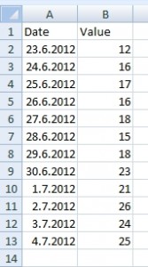
Let’s have a list of some values. The values are taken every day. The task is to create chart showing only last 5 days from today. Charts must be updated automatically.

Important: I wrote this on 4.7.2012, so for this example is 4.7.2012 the current date.

List of values by date
Continue reading “Automatic change in the chart according to the current date” »

Automatic change of data source in a pivot table

There is a problem with Pivot Table. When you add new row or column to source table, the pivot table won’t expand range. You must do it manually using menu “Change Data Source”. So this is the question, how can I do it automatically? Continue reading “Automatic change of data source in a pivot table” »

How to hide error values

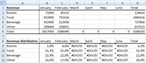
In Excel table may occur some error values like #DIV/0, #N/A … But it does not necessarily mean an error in a formula. It could mean that there is some unfilled value or some value is not in table and so on. In this cases is better display nothing or some specific word or number instead of error value.  I have prepared table containing #DIV/0 values and two ways how to solve it. The first is using formula and the second is made by conditional formatting.

Table with error values

The bottom table have simple formula for calculating percentage of items revenue. For example in B9 is formula =B2/B$6. So, when cells in the top table is empty, result of formula is #DIV/0. Continue reading “How to hide error values” »

Average with multiple conditions

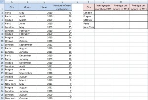
There is problem with average for some specific values in a table. We need to make average of the items that meet several criteria. Following table represents data of some worldwide company. You can see branch offices in the cities and number of their new customers per each month and year.

Average with multiple conditions example

 How to do average of specific branch offices for specific year? Continue reading “Average with multiple conditions” »

Address of the first empty cell in a row

In some cases it is useful to know the address of the first empty cell in a row. This is a way to do this without macros. Write the following formula and press CTRL+SHIFT+ENTER. Excel adds braces { } and saves it as array formula.

=ADDRESS(row number,COLUMN(INDEX(firstCell:lastCell,1,MATCH(TRUE,LEN(firstCell:lastCell)=0,0)))) Continue reading “Address of the first empty cell in a row” »

Address of the first empty cell in a column

In some cases it is useful to know the address of the first empty cell in a column. This is a way to do this without macros. Write the following formula and press CTRL+SHIFT+ENTER. Excel adds braces { } and saves it as array formula.

=ADDRESS(ROW(INDEX(firstCell:lastCell,
MATCH(TRUE,LEN(firstCell:lastCell)=0,0),1)),column number)

Continue reading “Address of the first empty cell in a column” »

Two tables with common column displayed in one chart

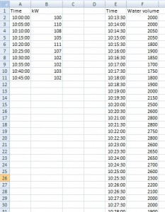
In this example we have data from some water pump. We were observed 2 variables (kW and water volume). So there are two data series measured in time, but in different time intervals. First measurement started at 10:00 and continued at 5 minute intervals (left table). Second measurement started at 10:13:30 and continued at half minute intervals (right table). We want Excel to show relationship between these two data series in one chart.

Tables with data series

How to show these tables in one chart? Solution

Number of rows that (not) contain a specific value

I prepared two ways to solve this problem. The first uses values in a new column and the second uses array formula. Both have their advantages.

Example

Table in the picture below contains information about the success of students making 3 exams. Value “Yes” means he passed, value “No” means he did not pass. Student should have value “Yes” in each column to pass all exams.

Rows not contain value - example1

How many students pass all of exams? The question is, how to count rows having value “Yes” in column B or C or D. Continue reading “Number of rows that (not) contain a specific value” »

Copyright © All Rights Reserved · Green Hope Theme by Sivan & schiy · Proudly powered by WordPress