How to highlight whole row using Conditional Formatting

Conditional formatting is very useful tool for highlighting cells in MS Excel. But there is the problem with coloring whole row or whole column of table. This example shows how to do that. Continue reading “How to highlight whole row using Conditional Formatting” »

How to highlight first Monday of the month in Excel table

Let’s have a list of dates or some kind of calendar. We want to highlight first Mondays or Tuesdays or Wednesdays etc. in each month. The example shows how to use conditional formatting to solve this task. Continue reading “How to highlight first Monday of the month in Excel table” »

Free sport training calendar

This training diary is designed for all kinds of sports. You can write the plan to the table and control its implementation and monitor your progress. The template is especially suitable for recording numbers of pushups, chin-ups, running, cycling miles (kilometers), pools, every fitness performances and many others sports activities. This Excel file offers weeks and months statistics of your training.

Continue reading “Free sport training calendar” »

How to highlight a specific day in the calendar

In this example, I will use conditional formatting to color weekends in the calendar. Let’s have following calendar for checking attendance.


Attendance calendar

Continue reading “How to highlight a specific day in the calendar” »

How to hide error values

In Excel table may occur some error values like #DIV/0, #N/A … But it does not necessarily mean an error in a formula. It could mean that there is some unfilled value or some value is not in table and so on. In this cases is better display nothing or some specific word or number instead of error value.  I have prepared table containing #DIV/0 values and two ways how to solve it. The first is using formula and the second is made by conditional formatting.
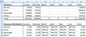
Table with error values

The bottom table have simple formula for calculating percentage of items revenue. For example in B9 is formula =B2/B$6. So, when cells in the top table is empty, result of formula is #DIV/0. Continue reading “How to hide error values” »

Conditional Formatting in column (bar) charts

Excel does not support conditional formatting in charts, but we can solve it with a little trick. Original data will be split into a new table and then will be displayed by Stacked Column chart. The result will look like conditional formatting.

Example

Let us have following data table. We want to highlight a column in chart having a value less than 20.

Source table - example1

Simple chart for this table looks like this:

Simple column chart - example1

How to automatically highlight columns? Continue reading “Conditional Formatting in column (bar) charts” »

Copyright © All Rights Reserved · Green Hope Theme by Sivan & schiy · Proudly powered by WordPress