How to exclude hidden rows in pivot table
Normally, pivot table counts the hidden rows. We have to add a flag to each row to determine if it is hidden or not. How to do that shows this example.
Example
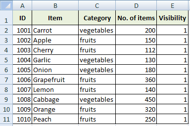
We have this common table including some items, categories and number of items. In the table is column visibility (value 1 is for visible row, value 0 is for hidden row).
Visibility values are made by formula:
=SUBTOTAL(103,A2)
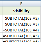
The first argument of SUBTOTAL function causes that SUBTOTAL will count number of cells that are not empty. Therefore, the second argument has to be the value that is always filled (for example ID, name, title or something like that). SUBTOTAL can ignore hidden values, so when the row is hidden the result of the formula is 0.
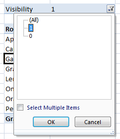
Now we create the Pivot Table and we put Visibility into Report Filter field.

Try hide some rows and use filter above the Pivot Table. Maybe, you will have to refresh the Pivot Table to see Visibility values 1 and 0.
I got this great idea to work perfectly as long as I put the pivot table in a new worksheet. For some reason it breaks down if I put the pivot table in the same worksheet. Not sure why.
Amazing ! thanks for the help bro. another sources told me to use excel macro. which is i’m not used to it, But using this method is way more simple
Simple solution of my problem with pivot tables. Thank you for this example.