How to highlight whole row using Conditional Formatting
Conditional formatting is very useful tool for highlighting cells in MS Excel. But there is the problem with coloring whole row or whole column of table. This example shows how to do that.
Example
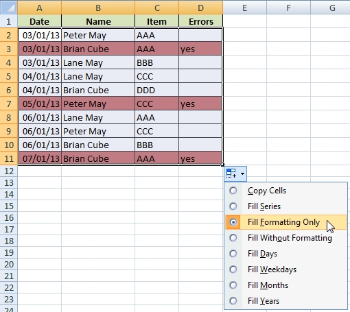
In this table, there is a list of inspections. The task is to color red the rows that contains errors (in the last column is “yes”).

Step 1 / New Formatting Rule
Select the first row of the table. Go to the Home >> Conditional Formatting >> New Rule… >> Select the choice Use a formula to determine which cells to format >> write the formula.
Formula for formatting row is =$D2=”yes”. The dollar sign ($) in the formula has to be only before the column (letter D). Reason is simple: We will copy the formatting and we want to vary the row number in the formula. So, there is no dollar sign ($) before the row number.

Step 2 / Copy formatting
You have two choices how to copy conditional formatting from the first row.
Use Format Painter
Select the first row >> go to the Home >> check the Format Painter >> select the rest of the table.

Use Auto fill
Select the first row >> Use the right bottom corner of the selection to copy values down. Don’t be afraid that values change, we fix it now. >> Click on the Auto Fill Options >> select Fill Formatting Only
I have an expiration date in my product table. I want to see which of these product are expirated. One option is highlighting rows by conditional formatting. It was a nightmare for me. Now it works ok. This explanation was really useful for me. How can I change the color. I want a specific color which will be representing my company.
I have a big checklist with a lot of important columns. I need more conditions then is showed in this simple example. How can I do that? Can you help me?
Hello,
yes it is possible 🙂 In the “Edit the Rule Description” section can be used advanced formulas or Excel functions. For example IF() function or combination of functions for more complex formula.
So you can write your conditions directly in this field or you can use other cell for evaluation.
Hi. That is great. Can you provide us some example of using IF function in conditional formatting?
I have been to 4 different websites and spent over an hour looking for help with this issue and this is the only explanation that worked for me. Thanks!!!
WOW, this is what I had looking for. Simple and easy explanation. Thanks.