How to display the current totals in the filter

Common Excel functions like SUM, AVERAGE, MAX, MIN or COUNT always calculate with the range of cells that you give to them. It does not matter if cells are visible or not. When we use the filter to select some of data, we want to calculate only the visible cells. There is one nice function called SUBTOTAL that solves this. It can replace 11 other functions and you can choose if it calculates hidden cells or not.

SUBTOTAL belongs to Math & Trig functions. Syntax is following:

SUBTOTAL(function_num, ref)

function_num parameter

This parameter decides which function will be used. It can be number  1 to 11 or number  101 to 111. In the official documentation is written that 1 to 11 includes hidden values and 101 to 111 ignores hidden values. It is not true when you use SUBTOTAL with the filter (filter does not “hide” cells). It is true when you use SUBTOTAL and Hide rows or columns (it’s not this case). So, it does not matter which format you write. In the official documentation is a nice table showing functions and their numbers:  https://office.microsoft.com/en-us/excel-help/subtotal-function-HP010062463.aspx. For example SUM has number 9 or 109,  AVERAGE has 1 or 101, MAX has 4 or 104 and MIN has 5 or 105.

ref parameter

This is the standard parameter for the range of cells. For example A1:C2 etc.

Example

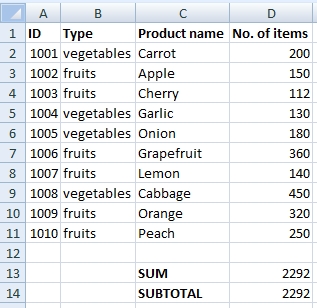
There is a list of fruits and vegetables we have on the warehouse. We use the filter to find out how many items of fruits we have (I know that fruits and vegetables unit is the weight, but there is lb, kg and others, so I used “items” to simplify the example).

Formulas:

=SUM(D2:D11)

=SUBTOTAL(9,D2:D11)

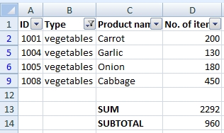
Now we filter the vegetables. SUM function calculates the whole table, but SUBTOTAL calculates only visible cells.

NOTE: Don’t place the SUBTOTAL function beside the table. Filter could hide it. It is better to place it above or below the table.